Trapped Ion vs Superconducting for QAOA at 100+ Qubits

QAOA at 100+ qubits reads well on a vendor slide and badly on a purchase order. The algorithm is simple to describe — alternating cost and mixer layers, one variational angle per layer — but its economics on real hardware are anything but. Every SWAP inserted to satisfy sparse connectivity multiplies two-qubit-gate count. Every two-qubit gate erodes fidelity. And the sampling budget needed to estimate the cost function scales with the noise, not the ideal problem.

That is why the trapped-ion versus superconducting choice cannot be settled by qubit count alone. A buyer running MaxCut, portfolio, or higher-order Ising instances between 100 and 156 logical variables is really choosing between two very different cost structures: expensive shots on a slow, high-fidelity, fully connected machine, or cheap shots on a fast, lossier, sparsely connected one. The right answer depends on circuit depth, connectivity of the problem graph, and how many samples the classical outer loop needs to converge.

Why QAOA Economics Differ From VQE

The VQE chemistry selection logic centred on ansatz expressibility and active-space size. QAOA at scale inverts those priorities. The ansatz is fixed by the problem Hamiltonian, so expressibility is not a knob. What matters is the per-shot cost of executing a circuit of depth p whose two-qubit-gate count grows linearly with the number of edges in the problem graph and, on nearest-neighbour hardware, further inflates through SWAP routing.

For a fully connected MaxCut instance on n qubits, the ideal circuit contains n(n−1)/2 two-qubit gates per QAOA layer. On an all-to-all machine, that count is native. On a heavy-hex or square-lattice device, the transpiler must route non-adjacent pairs through SWAP chains, and the effective gate count can rise by an order of magnitude before p=1 even completes. This is the single dominant variable in the procurement decision.

The Hardware In Contention

Four systems now cover the 80 to 156-qubit band with cloud access mature enough to underwrite a project. Two are trapped-ion, two are superconducting, and they price and perform on almost opposite curves.

Quantinuum H2 / Helios. The successor generation, Helios, is a 98-qubit trapped-ion processor built on the QCCD architecture using 137Ba+ hyperfine qubits, with all-to-all connectivity from a rotatable ion storage ring and average infidelities of 2.5×10⁻⁵ for single-qubit gates and 7.9×10⁻⁴ for two-qubit gates. Its predecessor H2-1 anchored the LR-QAOA benchmark that passed at 56 qubits by running three layers of LR-QAOA involving 4,620 two-qubit gates on a fully connected MaxCut circuit.

IonQ Forte Enterprise. A 36-qubit trapped-ion system with all-to-all connectivity, now generally available. Sub-100 qubits, so it is not the primary candidate for a 100-qubit workload, but included here because IonQ is the reference trapped-ion price point on Braket and any 100-qubit-class successor will inherit that curve.

IBM Heron R2. A 156-qubit superconducting device with fixed-frequency transmon qubits arranged on a heavy-hex lattice with tunable couplers, reporting typical two-qubit gate errors below 10⁻³ and CLOPS above 2×10⁵. Nearest-neighbour connectivity of maximum degree 3.

Rigetti Ankaa-3. An 84-qubit superconducting device on a square lattice with tunable couplers, reporting 99.5% median two-qubit gate fidelity on fSim gates with a 56-nanosecond median gate time. Below the 100-qubit threshold, but priced far under the trapped-ion tier and worth benchmarking against a partitioned instance.

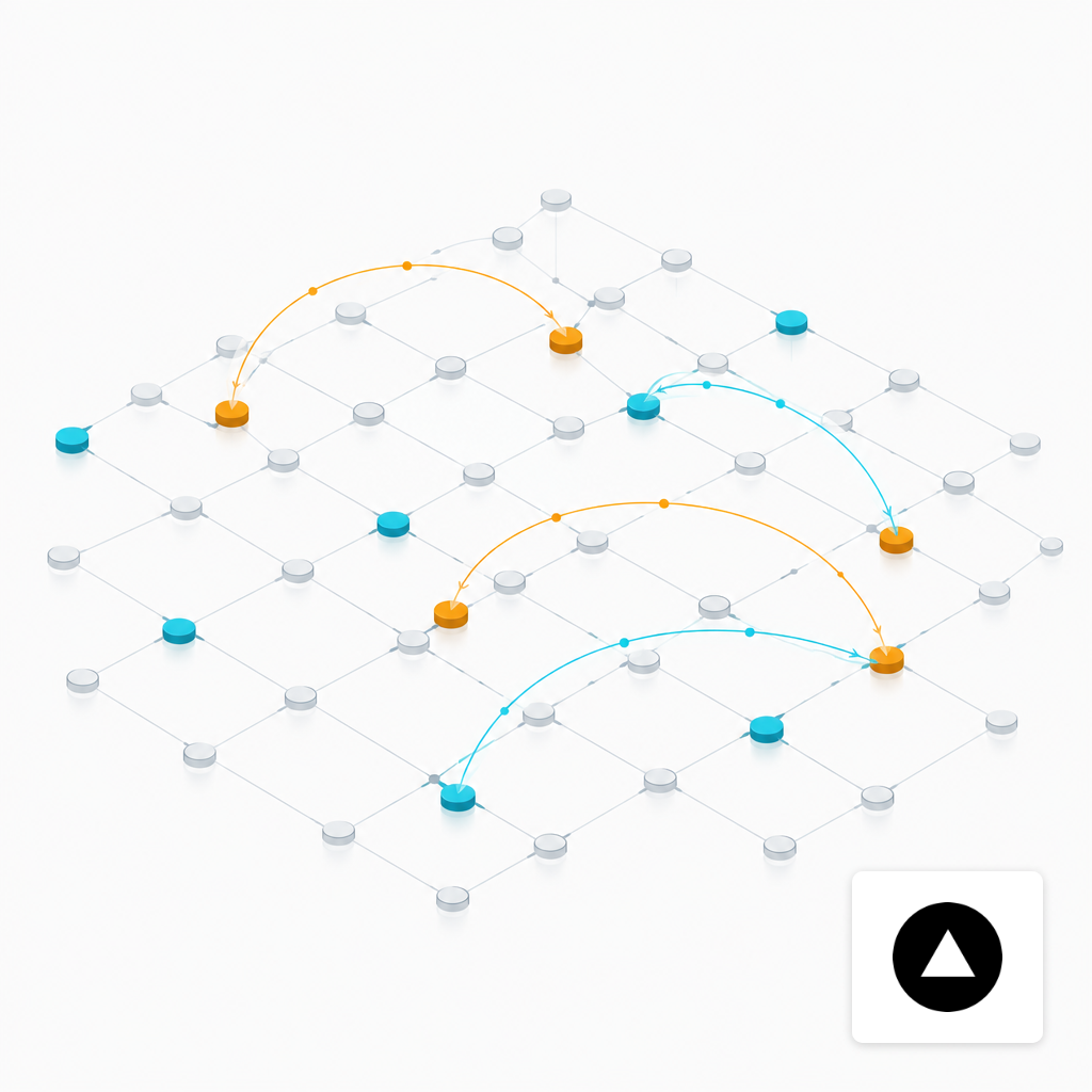
Fidelity Sets The Depth Ceiling, Not The Qubit Count

The two-qubit error rate compounds. For a circuit of N₂Q two-qubit gates and per-gate error ε, an independent-error estimate of process fidelity is (1−ε)^N₂Q. At Heron R2's sub-10⁻³ error rate, a circuit with 1,000 two-qubit gates has an estimated fidelity around 0.37; at 3,000 gates, roughly 0.05. Quantinuum's 7.9×10⁻⁴ two-qubit infidelity on Helios pushes those crossovers modestly further, but the real advantage is that a fully connected instance needs no SWAP inflation at all.

Empirically, the picture matches the arithmetic. IonQ Aria-1 and Forte-1 achieved the highest fidelities, success probabilities, and approximation ratios in a cross-platform QAOA benchmark, attributed to native all-to-all connectivity and low two-qubit gate errors, while IQM Garnet and Rigetti Ankaa-3 delivered faster gate execution but accumulated more error in deeper circuits. On the IBM side, a scaling study of QAOA on higher-order Ising models found the best 127-qubit processors improved solution quality only up to p=2 before degrading, while 27-qubit devices improved up to p=3 at equivalent CNOT depth. Depth headroom on superconducting hardware is real but shallow.

That does not automatically favour ions. IBM's LR-QAOA run on ibm_fez pushed a 100-qubit problem through up to 10,000 layers with coherent information persisting until roughly 300 layers, at 21 seconds of QPU time for 1,000 samples of the p=10,000 circuit. Superconducting hardware can execute far more shots per unit time; whether those shots carry useful signal depends on where the noise floor sits for the specific problem.

Shot-Rate And Per-Shot Pricing Decide The Bill

The commercial gap is stark. On AWS Braket, per-task pricing is uniform, but per-shot pricing varies by more than 180× across devices, with a 10,000-shot IonQ Forte circuit landing near $800 and the equivalent on Rigetti Cepheus near $5. That ratio is not primarily a fidelity story; it is a throughput story. Trapped-ion two-qubit gates run in hundreds of microseconds. Superconducting two-qubit gates run in tens of nanoseconds. The provider prices what it can serve.

For a QAOA outer loop that needs, say, 5,000 shots per parameter evaluation and 200 evaluations to converge, the difference between $0.08 per shot and sub-cent per shot is the difference between a five-figure and a three-figure run. IBM sits on a different meter entirely: per-minute Qiskit Runtime rather than per-shot Braket, which shifts optimization from minimizing shots to minimizing wall-clock QPU time, including transpile-side overhead.

A Procurement Decision Rule

The choice reduces to two questions. First: does the problem graph have dense connectivity relative to the hardware? Second: how many shots does the classical outer loop actually need to converge to a useful approximation ratio?

A dense graph on 100+ variables — a fully connected MaxCut, a portfolio covariance matrix, a QUBO with high edge density — inflates the two-qubit gate count on nearest-neighbour hardware by roughly a factor equal to the average routing distance. On heavy-hex, that factor can exceed 5× for random dense problems. In that regime, the trapped-ion fidelity and connectivity premium is often recovered in fewer required shots, because higher per-shot fidelity means higher probability mass on the true optimum. A sparse graph that maps naturally onto a heavy-hex or square lattice inverts the answer.

1. 11. Characterise the problem graph1 · Edge density and average routing distance on the candidate topology
2. 22. Estimate the compiled 2Q gate count2 · Native gates plus SWAP inflation at p=1, extrapolated to target depth
3. 33. Derive the depth ceiling from fidelity3 · (1 - epsilon)^N2Q to find where signal collapses
4. 44. Size the shot budget per evaluation4 · Shots x outer-loop iterations, scaled by noise floor
5. 55. Price it on both meters5 · Per-shot (Braket) versus per-minute (Qiskit Runtime)

What To Verify Before Committing

Vendor spec sheets are calibration snapshots, not procurement contracts. Median two-qubit fidelity is a distribution, and QAOA circuits sample all of it. Real-time layout selection matters: on Heron devices, dynamic chain selection based on layer fidelity is standard practice for the best published results, and it is a nontrivial operator skill. Ion machines list infidelity as a running average across the register, but chain reconfiguration overhead on QCCD adds wall-clock time that a per-shot price does not surface.

Independent aggregation helps. Cross-vendor QPU benchmark data and the modality breakdowns in the quantum computing architectures catalogue let a buyer compare calibration-adjusted figures rather than press-release medians, and current QPU availability across cloud providers determines whether a system is bookable inside a project timeline.

Where This Leaves The 100-Qubit Buyer

For a dense QAOA workload at 100 or more variables today, the defensible default is Quantinuum Helios or its H2 predecessor: fewer shots at higher unit cost, but the shots carry more signal and the connectivity is native. For a sparse-graph workload that fits the hardware topology, IBM Heron R2 delivers depth headroom and shot throughput at per-minute economics that reward tight compile-side optimization. Rigetti Ankaa-3 is the low-cost benchmark; sub-100 qubits, but the correct comparison point for cost-per-approximation-ratio at partitioned instance sizes. IonQ Forte Enterprise sits in the same trapped-ion economic tier as Helios but at a lower qubit count, so it enters the 100-qubit conversation only once its successor reaches that scale.

Two-qubit fidelity is the ceiling. Connectivity is the multiplier. Per-shot price is the meter. A buyer who has all three numbers written down before running the first job is a buyer with a defensible procurement decision.